This can be seen as a natural extension of polynomial approximations. The latter are
used in numerous applications where there role is, for example, to replace expensive
simulations with cheap to evaluate function calls. This is especially amenable for the task
of parameter-space exploration with numerical methods and data comparison.
The motivation behind this work is to overcome the limitations of the applicability of
polynomial approximations.
Examples (click for animation)
In this example we compare polynomial (left) and rational approximations (right) and how they compare to
the to be interpolated data-set. In the animation, higher and higher polynomial orders (m for the numerator, n for the denominator)
are used.The legend also reports the total number of coefficients (Ncoeff) that is the number of fit parameters
(and therefore input data) are required to calculate a solution to the approximation problem. As becomes
clear very quickly, the rational approximations give a much better fit of the data with fewer coefficients that need to be determined.
Interpolation of a 1D dataset with polynomial approximations. Very high polynomial orders are required to obtain an acceptable fit of the data.

Interpolating the same data with rational approximations gives a much better fit with less required input data,
Application to likelihood scan
This is a (toy) representation of an application where we want to find regions in a 3D parameter-space of a certain physics model that are compatible with data. One measure often used for such a task is a likelihood function defined as
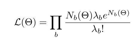
where theta is a point in the parameter space and the product runs of bins of histogrammed data. The Nb are the predicted counts coming from either the full simulation or an approximation to it while the lambdab represent the experimentally measured counts.
The plot on the left shows the “true” result of the likelihood contour obtained when running the expensive simulation. The center plots shows the result obtained when replacing the calls to the expensive simulation with those of the cheap rational approximation. As can be seen, the agreement is excellent. For completeness, the plot on the right shows what happens if polynomial approximations are used. They cleary are unable to capture the true physics behaviour of the underlying simulation.
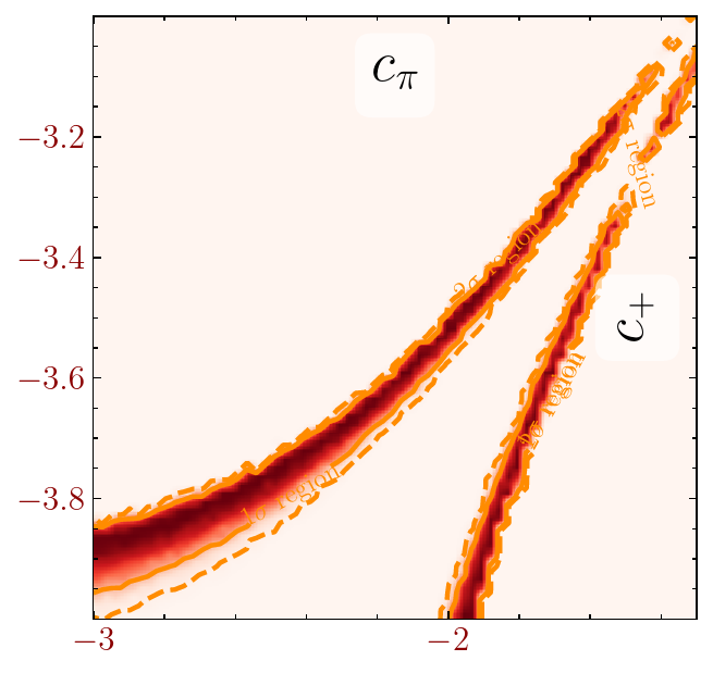
Result obtained without approximation (i.e. full simulation used to calculated L at every point p).

Result obtained using our rational approximations.

Result obtained when using purely polynomial approximations.